A student asked me a really interesting question recently; a pair of questions, really. We have just discussed the correlation coefficient as a measure of the direction/strength of a linear association between two quantitative variables, and I demonstrated in class that the calculation for this quantity, referred to by the letter r, can be found by the formula

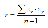
In other words, for each point of a scatterplot, find the z-score for the x-coordinate and the y-coordinate of that point and multiply those together. Do this for all of the points in your scatterplot, add them together, and divide by n-1 to get your correlation coefficient.

We discussed various properties of this quantity, and my student asked me that question that teachers always hope for (if not without a bit of dread sometimes!): “Why?” Why does this formula produce a quantity that measures the strength of a linear association? Also, why must the value of r necessarily be bound between -1 and 1? In this post, I seek to start an answer to these questions.

The correlation coefficient that we use in AP Statistics is actually something called the PCC or Pearson Correlation Coefficient (or, if you really want to impress your friends, the “Pearson Product-Moment Correlation Coefficient” or PPMCC). The formula for this value can be expressed in a number of different ways, and the version above is probably the most succinct. But probably most conventionally, the formula for the PCC of a sample of data is generally given as:

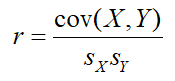
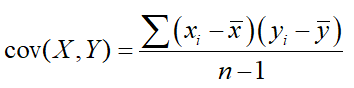
where the values in the denominators represent the standard deviations of the variables on the x- and y-axis, and cov(X,Y) represents the covariance of the two variables. The covariance of a sample is a measure of the joint variability of the two variables in that sample, and is found with the formula:

In general, if you find that the values of your explanatory (x-axis) and response (y-axis) variables both tend to be above average and below average for the same cases, your covariance will wind up being positive. If your explanatory is above average when your response is below average and vice-versa, the covariance will be negative.

For example, on days when temperatures in Ithaca are above the yearly average, temperatures in Cape Town, South Africa are below the yearly average, since summer in Ithaca corresponds to winter in Cape Town. Take a sample of temperatures over the whole year, and that sample will have a negative covariance. Similarly, the covariance of a sample of temperature data taken from Ithaca and Zurich, Switzerland will be positive, as those two cities see summer and winter in the same months. The magnitude of the covariance might be more extreme for one pair or the other — perhaps temperatures in Zurich vary more widely than temperatures in Cape Town — but the sign of the covariance should be clear.

The unit of the covariance is the product of the units that the explanatory and response variables are measured in and its magnitude is completely dependent on how much variability occurs in the those variables. Imagine you’re trying to measure the strengths of associations between fuel efficiency for cars versus other various measurements. Compare fuel efficiency to the weight of the car, and you’ll get “Pound-MPGs.” Compare fuel efficiency to tire pressure, and you’ll get “PSI-MPGs.” Since the weights of cars are larger numbers, measured in thousands of pounds, and the tire pressure of cars tend to be numbers between 20 and 40 PSI, the magnitude of the covariances for these two associations will be wildly different from each other. So how do we assess which comparison produces a stronger association?

This is what the correlation coefficient does. By dividing the covariance by the product of the standard deviations as we saw in Formula 2 above, we are, for one, dividing by a quantity also measured in the product of units for the explanatory and response variables, thus giving us a unitless (“dimensionless“) quantity. But more importantly, this action serves to normalize the covariance by including an accounting of the magnitude of the variability for each individual variable in tandem with the amount of joint variability between both. Thus, we have a value that is more easily compared for multiple different associations, and one that we can more easily evaluate on its own.

But why is the correlation coefficient bound between -1 and 1? And why does a value of r near 0 indicate a weak association while a value near one of the extremes indicate a strong association? Please read on!